DPWX/Microburst winds and melting hail at the Easton Airport field site: 9 July 2015: Difference between revisions
Pat kennedy (talk | contribs) No edit summary |
(Added reference links and article categories) |
||
| Line 1: | Line 1: | ||
==Overview== | ==Overview== | ||
During the late afternoon and early evening hours of 9 July 2015 (local date) the CSU-CHILL conducted continuous 1.5 degree elevation angle 360 degree PPI scans to collect low altitude dual polarization radar observations of precipitation at the instrumentation site located at the Easton Valley View Airport (azimuth 171.4 deg / range 13 km from CHILL). This site was established in the fall of 2014 to support the Multi-Angle Snow Camera and Radar (MASCRAD) project | During the late afternoon and early evening hours of 9 July 2015 (local date) the CSU-CHILL conducted continuous 1.5 degree elevation angle 360 degree PPI scans to collect low altitude dual polarization radar observations of precipitation at the instrumentation site located at the Easton Valley View Airport (azimuth 171.4 deg / range 13 km from CHILL). This site was established in the fall of 2014 to support the Multi-Angle Snow Camera and Radar ([[DPWX/Initial_Multiple_Angle_Snow_Camera-Radar_Experiment_(MASCRAD)_Project_Operations:_15_November_2014|MASCRAD]]) project | ||
==Reflectivity loop== | ==Reflectivity loop== | ||
| Line 7: | Line 7: | ||
<center> | <center> | ||
<imgloop delay=300 imgprefix="http://www.chill.colostate.edu/anim/aug_2015_EVV_uburst/" width=640 height=512> | <imgloop delay=300 imgprefix="http://www.chill.colostate.edu/anim/aug_2015_EVV_uburst/" width=640 height=512> | ||
dBZ.CHL20150709_234247 GFC_1 PPI Sweep 01 Plot 0.png | dBZ.CHL20150709_234247 GFC_1 PPI Sweep 01 Plot 0.png|23:42:47 UTC | ||
dBZ.CHL20150709_234419 GFC_1 PPI Sweep 01 Plot 0.png | dBZ.CHL20150709_234419 GFC_1 PPI Sweep 01 Plot 0.png|23:44:19 UTC | ||
dBZ.CHL20150709_234551 GFC_1 PPI Sweep 01 Plot 0.png | dBZ.CHL20150709_234551 GFC_1 PPI Sweep 01 Plot 0.png|23:45:51 UTC | ||
dBZ.CHL20150709_234722 GFC_1 PPI Sweep 01 Plot 0.png | dBZ.CHL20150709_234722 GFC_1 PPI Sweep 01 Plot 0.png|23:47:22 UTC | ||
dBZ.CHL20150709_234854 GFC_1 PPI Sweep 01 Plot 0.png | dBZ.CHL20150709_234854 GFC_1 PPI Sweep 01 Plot 0.png|23:48:54 UTC | ||
dBZ.CHL20150709_235025 GFC_1 PPI Sweep 01 Plot 0.png | dBZ.CHL20150709_235025 GFC_1 PPI Sweep 01 Plot 0.png|23:50:25 UTC | ||
dBZ.CHL20150709_235157 GFC_1 PPI Sweep 01 Plot 0.png | dBZ.CHL20150709_235157 GFC_1 PPI Sweep 01 Plot 0.png|23:51:57 UTC | ||
dBZ.CHL20150709_235329 GFC_1 PPI Sweep 01 Plot 0.png | dBZ.CHL20150709_235329 GFC_1 PPI Sweep 01 Plot 0.png|23:53:29 UTC | ||
dBZ.CHL20150709_235500 GFC_1 PPI Sweep 01 Plot 0.png | dBZ.CHL20150709_235500 GFC_1 PPI Sweep 01 Plot 0.png|23:55:00 UTC | ||
dBZ.CHL20150709_235632 GFC_1 PPI Sweep 01 Plot 0.png | dBZ.CHL20150709_235632 GFC_1 PPI Sweep 01 Plot 0.png|23:56:32 UTC | ||
dBZ.CHL20150709_235803 GFC_1 PPI Sweep 01 Plot 0.png | dBZ.CHL20150709_235803 GFC_1 PPI Sweep 01 Plot 0.png|23:58:03 UTC | ||
dBZ.CHL20150709_235935 GFC_1 PPI Sweep 01 Plot 0.png | dBZ.CHL20150709_235935 GFC_1 PPI Sweep 01 Plot 0.png|23:59:35 UTC | ||
dBZ.CHL20150710_000106 GFC_1 PPI Sweep 01 Plot 0.png | dBZ.CHL20150710_000106 GFC_1 PPI Sweep 01 Plot 0.png|00:01:06 UTC | ||
dBZ.CHL20150710_000238 GFC_1 PPI Sweep 01 Plot 0.png | dBZ.CHL20150710_000238 GFC_1 PPI Sweep 01 Plot 0.png|00:02:38 UTC | ||
dBZ.CHL20150710_000410 GFC_1 PPI Sweep 01 Plot 0.png | dBZ.CHL20150710_000410 GFC_1 PPI Sweep 01 Plot 0.png|00:04:10 UTC | ||
dBZ.CHL20150710_000541 GFC_1 PPI Sweep 01 Plot 0.png | dBZ.CHL20150710_000541 GFC_1 PPI Sweep 01 Plot 0.png|00:05:41 UTC | ||
dBZ.CHL20150710_000713 GFC_1 PPI Sweep 01 Plot 0.png | dBZ.CHL20150710_000713 GFC_1 PPI Sweep 01 Plot 0.png|00:07:13 UTC | ||
dBZ.CHL20150710_000844 GFC_1 PPI Sweep 01 Plot 0.png | dBZ.CHL20150710_000844 GFC_1 PPI Sweep 01 Plot 0.png|00:08:44 UTC | ||
dBZ.CHL20150710_001016 GFC_1 PPI Sweep 01 Plot 0.png | dBZ.CHL20150710_001016 GFC_1 PPI Sweep 01 Plot 0.png|00:10:16 UTC | ||
dBZ.CHL20150710_001148 GFC_1 PPI Sweep 01 Plot 0.png | dBZ.CHL20150710_001148 GFC_1 PPI Sweep 01 Plot 0.png|00:11:48 UTC | ||
dBZ.CHL20150710_001319 GFC_1 PPI Sweep 01 Plot 0.png | dBZ.CHL20150710_001319 GFC_1 PPI Sweep 01 Plot 0.png|00:13:19 UTC | ||
dBZ.CHL20150710_001451 GFC_1 PPI Sweep 01 Plot 0.png | dBZ.CHL20150710_001451 GFC_1 PPI Sweep 01 Plot 0.png|00:14:51 UTC | ||
dBZ.CHL20150710_001622 GFC_1 PPI Sweep 01 Plot 0.png | dBZ.CHL20150710_001622 GFC_1 PPI Sweep 01 Plot 0.png|00:16:22 UTC | ||
dBZ.CHL20150710_001754 GFC_1 PPI Sweep 01 Plot 0.png | dBZ.CHL20150710_001754 GFC_1 PPI Sweep 01 Plot 0.png|00:17:54 UTC | ||
dBZ.CHL20150710_001926 GFC_1 PPI Sweep 01 Plot 0.png | dBZ.CHL20150710_001926 GFC_1 PPI Sweep 01 Plot 0.png|00:19:26 UTC | ||
dBZ.CHL20150710_002057 GFC_1 PPI Sweep 01 Plot 0.png | dBZ.CHL20150710_002057 GFC_1 PPI Sweep 01 Plot 0.png|00:20:57 UTC | ||
dBZ.CHL20150710_002229 GFC_1 PPI Sweep 01 Plot 0.png | dBZ.CHL20150710_002229 GFC_1 PPI Sweep 01 Plot 0.png|00:22:29 UTC | ||
dBZ.CHL20150710_002400 GFC_1 PPI Sweep 01 Plot 0.png | dBZ.CHL20150710_002400 GFC_1 PPI Sweep 01 Plot 0.png|00:24:00 UTC | ||
dBZ.CHL20150710_002532 GFC_1 PPI Sweep 01 Plot 0.png | dBZ.CHL20150710_002532 GFC_1 PPI Sweep 01 Plot 0.png|00:25:32 UTC | ||
dBZ.CHL20150710_002703 GFC_1 PPI Sweep 01 Plot 0.png | dBZ.CHL20150710_002703 GFC_1 PPI Sweep 01 Plot 0.png|00:27:03 UTC | ||
dBZ.CHL20150710_002835 GFC_1 PPI Sweep 01 Plot 0.png | dBZ.CHL20150710_002835 GFC_1 PPI Sweep 01 Plot 0.png|00:28:35 UTC | ||
dBZ.CHL20150710_003007 GFC_1 PPI Sweep 01 Plot 0.png | dBZ.CHL20150710_003007 GFC_1 PPI Sweep 01 Plot 0.png|00:30:07 UTC | ||
dBZ.CHL20150710_003138 GFC_1 PPI Sweep 01 Plot 0.png | dBZ.CHL20150710_003138 GFC_1 PPI Sweep 01 Plot 0.png|00:31:38 UTC | ||
dBZ.CHL20150710_003310 GFC_1 PPI Sweep 01 Plot 0.png | dBZ.CHL20150710_003310 GFC_1 PPI Sweep 01 Plot 0.png|00:33:10 UTC | ||
dBZ.CHL20150710_003441 GFC_1 PPI Sweep 01 Plot 0.png | dBZ.CHL20150710_003441 GFC_1 PPI Sweep 01 Plot 0.png|00:34:41 UTC | ||
dBZ.CHL20150710_003613 GFC_1 PPI Sweep 01 Plot 0.png | dBZ.CHL20150710_003613 GFC_1 PPI Sweep 01 Plot 0.png|00:36:13 UTC | ||
dBZ.CHL20150710_003745 GFC_1 PPI Sweep 01 Plot 0.png | dBZ.CHL20150710_003745 GFC_1 PPI Sweep 01 Plot 0.png|00:37:45 UTC | ||
dBZ.CHL20150710_003916 GFC_1 PPI Sweep 01 Plot 0.png | dBZ.CHL20150710_003916 GFC_1 PPI Sweep 01 Plot 0.png|00:39:16 UTC | ||
dBZ.CHL20150710_004048 GFC_1 PPI Sweep 01 Plot 0.png | dBZ.CHL20150710_004048 GFC_1 PPI Sweep 01 Plot 0.png|00:40:48 UTC | ||
dBZ.CHL20150710_004219 GFC_1 PPI Sweep 01 Plot 0.png | dBZ.CHL20150710_004219 GFC_1 PPI Sweep 01 Plot 0.png|00:42:19 UTC | ||
dBZ.CHL20150710_004351 GFC_1 PPI Sweep 01 Plot 0.png | dBZ.CHL20150710_004351 GFC_1 PPI Sweep 01 Plot 0.png|00:43:51 UTC | ||
dBZ.CHL20150710_004522 GFC_1 PPI Sweep 01 Plot 0.png | dBZ.CHL20150710_004522 GFC_1 PPI Sweep 01 Plot 0.png|00:45:22 UTC | ||
dBZ.CHL20150710_004654 GFC_1 PPI Sweep 01 Plot 0.png | dBZ.CHL20150710_004654 GFC_1 PPI Sweep 01 Plot 0.png|00:46:54 UTC | ||
dBZ.CHL20150710_004826 GFC_1 PPI Sweep 01 Plot 0.png | dBZ.CHL20150710_004826 GFC_1 PPI Sweep 01 Plot 0.png|00:48:26 UTC | ||
dBZ.CHL20150710_004957 GFC_1 PPI Sweep 01 Plot 0.png | dBZ.CHL20150710_004957 GFC_1 PPI Sweep 01 Plot 0.png|00:49:57 UTC | ||
dBZ.CHL20150710_005129 GFC_1 PPI Sweep 01 Plot 0.png | dBZ.CHL20150710_005129 GFC_1 PPI Sweep 01 Plot 0.png|00:51:29 UTC | ||
</imgloop> | </imgloop> | ||
</center> | </center> | ||
| Line 61: | Line 61: | ||
<center> | <center> | ||
<imgloop delay=300 imgprefix="http://www.chill.colostate.edu/anim/aug_2015_EVV_uburst/" width=640 height=512> | <imgloop delay=300 imgprefix="http://www.chill.colostate.edu/anim/aug_2015_EVV_uburst/" width=640 height=512> | ||
Vel.CHL20150709_234247 GFC_1 PPI Sweep 01 Plot 0.png | Vel.CHL20150709_234247 GFC_1 PPI Sweep 01 Plot 0.png|23:42:47 UTC | ||
Vel.CHL20150709_234419 GFC_1 PPI Sweep 01 Plot 0.png | Vel.CHL20150709_234419 GFC_1 PPI Sweep 01 Plot 0.png|23:44:19 UTC | ||
Vel.CHL20150709_234551 GFC_1 PPI Sweep 01 Plot 0.png | Vel.CHL20150709_234551 GFC_1 PPI Sweep 01 Plot 0.png|23:45:51 UTC | ||
Vel.CHL20150709_234722 GFC_1 PPI Sweep 01 Plot 0.png | Vel.CHL20150709_234722 GFC_1 PPI Sweep 01 Plot 0.png|23:47:22 UTC | ||
Vel.CHL20150709_234854 GFC_1 PPI Sweep 01 Plot 0.png | Vel.CHL20150709_234854 GFC_1 PPI Sweep 01 Plot 0.png|23:48:54 UTC | ||
Vel.CHL20150709_235025 GFC_1 PPI Sweep 01 Plot 0.png | Vel.CHL20150709_235025 GFC_1 PPI Sweep 01 Plot 0.png|23:50:25 UTC | ||
Vel.CHL20150709_235157 GFC_1 PPI Sweep 01 Plot 0.png | Vel.CHL20150709_235157 GFC_1 PPI Sweep 01 Plot 0.png|23:51:57 UTC | ||
Vel.CHL20150709_235329 GFC_1 PPI Sweep 01 Plot 0.png | Vel.CHL20150709_235329 GFC_1 PPI Sweep 01 Plot 0.png|23:53:29 UTC | ||
Vel.CHL20150709_235500 GFC_1 PPI Sweep 01 Plot 0.png | Vel.CHL20150709_235500 GFC_1 PPI Sweep 01 Plot 0.png|23:55:00 UTC | ||
Vel.CHL20150709_235632 GFC_1 PPI Sweep 01 Plot 0.png | Vel.CHL20150709_235632 GFC_1 PPI Sweep 01 Plot 0.png|23:56:32 UTC | ||
Vel.CHL20150709_235803 GFC_1 PPI Sweep 01 Plot 0.png | Vel.CHL20150709_235803 GFC_1 PPI Sweep 01 Plot 0.png|23:58:03 UTC | ||
Vel.CHL20150709_235935 GFC_1 PPI Sweep 01 Plot 0.png | Vel.CHL20150709_235935 GFC_1 PPI Sweep 01 Plot 0.png|23:59:35 UTC | ||
Vel.CHL20150710_000106 GFC_1 PPI Sweep 01 Plot 0.png | Vel.CHL20150710_000106 GFC_1 PPI Sweep 01 Plot 0.png|00:01:06 UTC | ||
Vel.CHL20150710_000238 GFC_1 PPI Sweep 01 Plot 0.png | Vel.CHL20150710_000238 GFC_1 PPI Sweep 01 Plot 0.png|00:02:38 UTC | ||
Vel.CHL20150710_000410 GFC_1 PPI Sweep 01 Plot 0.png | Vel.CHL20150710_000410 GFC_1 PPI Sweep 01 Plot 0.png|00:04:10 UTC | ||
Vel.CHL20150710_000541 GFC_1 PPI Sweep 01 Plot 0.png | Vel.CHL20150710_000541 GFC_1 PPI Sweep 01 Plot 0.png|00:05:41 UTC | ||
Vel.CHL20150710_000713 GFC_1 PPI Sweep 01 Plot 0.png | Vel.CHL20150710_000713 GFC_1 PPI Sweep 01 Plot 0.png|00:07:13 UTC | ||
Vel.CHL20150710_000844 GFC_1 PPI Sweep 01 Plot 0.png | Vel.CHL20150710_000844 GFC_1 PPI Sweep 01 Plot 0.png|00:08:44 UTC | ||
Vel.CHL20150710_001016 GFC_1 PPI Sweep 01 Plot 0.png | Vel.CHL20150710_001016 GFC_1 PPI Sweep 01 Plot 0.png|00:10:16 UTC | ||
Vel.CHL20150710_001148 GFC_1 PPI Sweep 01 Plot 0.png | Vel.CHL20150710_001148 GFC_1 PPI Sweep 01 Plot 0.png|00:11:48 UTC | ||
Vel.CHL20150710_001319 GFC_1 PPI Sweep 01 Plot 0.png | Vel.CHL20150710_001319 GFC_1 PPI Sweep 01 Plot 0.png|00:13:19 UTC | ||
Vel.CHL20150710_001451 GFC_1 PPI Sweep 01 Plot 0.png | Vel.CHL20150710_001451 GFC_1 PPI Sweep 01 Plot 0.png|00:14:51 UTC | ||
Vel.CHL20150710_001622 GFC_1 PPI Sweep 01 Plot 0.png | Vel.CHL20150710_001622 GFC_1 PPI Sweep 01 Plot 0.png|00:16:22 UTC | ||
Vel.CHL20150710_001754 GFC_1 PPI Sweep 01 Plot 0.png | Vel.CHL20150710_001754 GFC_1 PPI Sweep 01 Plot 0.png|00:17:54 UTC | ||
Vel.CHL20150710_001926 GFC_1 PPI Sweep 01 Plot 0.png | Vel.CHL20150710_001926 GFC_1 PPI Sweep 01 Plot 0.png|00:19:26 UTC | ||
Vel.CHL20150710_002057 GFC_1 PPI Sweep 01 Plot 0.png | Vel.CHL20150710_002057 GFC_1 PPI Sweep 01 Plot 0.png|00:20:57 UTC | ||
Vel.CHL20150710_002229 GFC_1 PPI Sweep 01 Plot 0.png | Vel.CHL20150710_002229 GFC_1 PPI Sweep 01 Plot 0.png|00:22:29 UTC | ||
Vel.CHL20150710_002400 GFC_1 PPI Sweep 01 Plot 0.png | Vel.CHL20150710_002400 GFC_1 PPI Sweep 01 Plot 0.png|00:24:00 UTC | ||
Vel.CHL20150710_002532 GFC_1 PPI Sweep 01 Plot 0.png | Vel.CHL20150710_002532 GFC_1 PPI Sweep 01 Plot 0.png|00:25:32 UTC | ||
Vel.CHL20150710_002703 GFC_1 PPI Sweep 01 Plot 0.png | Vel.CHL20150710_002703 GFC_1 PPI Sweep 01 Plot 0.png|00:27:03 UTC | ||
Vel.CHL20150710_002835 GFC_1 PPI Sweep 01 Plot 0.png | Vel.CHL20150710_002835 GFC_1 PPI Sweep 01 Plot 0.png|00:28:35 UTC | ||
Vel.CHL20150710_003007 GFC_1 PPI Sweep 01 Plot 0.png | Vel.CHL20150710_003007 GFC_1 PPI Sweep 01 Plot 0.png|00:30:07 UTC | ||
Vel.CHL20150710_003138 GFC_1 PPI Sweep 01 Plot 0.png | Vel.CHL20150710_003138 GFC_1 PPI Sweep 01 Plot 0.png|00:31:38 UTC | ||
Vel.CHL20150710_003310 GFC_1 PPI Sweep 01 Plot 0.png | Vel.CHL20150710_003310 GFC_1 PPI Sweep 01 Plot 0.png|00:33:10 UTC | ||
Vel.CHL20150710_003441 GFC_1 PPI Sweep 01 Plot 0.png | Vel.CHL20150710_003441 GFC_1 PPI Sweep 01 Plot 0.png|00:34:41 UTC | ||
Vel.CHL20150710_003613 GFC_1 PPI Sweep 01 Plot 0.png | Vel.CHL20150710_003613 GFC_1 PPI Sweep 01 Plot 0.png|00:36:13 UTC | ||
Vel.CHL20150710_003745 GFC_1 PPI Sweep 01 Plot 0.png | Vel.CHL20150710_003745 GFC_1 PPI Sweep 01 Plot 0.png|00:37:45 UTC | ||
Vel.CHL20150710_003916 GFC_1 PPI Sweep 01 Plot 0.png | Vel.CHL20150710_003916 GFC_1 PPI Sweep 01 Plot 0.png|00:39:16 UTC | ||
Vel.CHL20150710_004048 GFC_1 PPI Sweep 01 Plot 0.png | Vel.CHL20150710_004048 GFC_1 PPI Sweep 01 Plot 0.png|00:40:48 UTC | ||
Vel.CHL20150710_004219 GFC_1 PPI Sweep 01 Plot 0.png | Vel.CHL20150710_004219 GFC_1 PPI Sweep 01 Plot 0.png|00:42:19 UTC | ||
Vel.CHL20150710_004351 GFC_1 PPI Sweep 01 Plot 0.png | Vel.CHL20150710_004351 GFC_1 PPI Sweep 01 Plot 0.png|00:43:51 UTC | ||
Vel.CHL20150710_004522 GFC_1 PPI Sweep 01 Plot 0.png | Vel.CHL20150710_004522 GFC_1 PPI Sweep 01 Plot 0.png|00:45:22 UTC | ||
Vel.CHL20150710_004654 GFC_1 PPI Sweep 01 Plot 0.png | Vel.CHL20150710_004654 GFC_1 PPI Sweep 01 Plot 0.png|00:46:54 UTC | ||
Vel.CHL20150710_004826 GFC_1 PPI Sweep 01 Plot 0.png | Vel.CHL20150710_004826 GFC_1 PPI Sweep 01 Plot 0.png|00:48:26 UTC | ||
Vel.CHL20150710_004957 GFC_1 PPI Sweep 01 Plot 0.png | Vel.CHL20150710_004957 GFC_1 PPI Sweep 01 Plot 0.png|00:49:57 UTC | ||
Vel.CHL20150710_005129 GFC_1 PPI Sweep 01 Plot 0.png | Vel.CHL20150710_005129 GFC_1 PPI Sweep 01 Plot 0.png|00:51:29 UTC | ||
</imgloop> | </imgloop> | ||
</center> | </center> | ||
==Dual polarization radar indications of hail at 9 | ==Dual polarization radar indications of hail at 9 GHz (X-band)== | ||
The CSU-CHILL radar's dual frequency feed horn allows the 9.5 m diameter main reflector to be shared by the 3 | The CSU-CHILL radar's dual frequency feed horn allows the 9.5 m diameter main reflector to be shared by the 3 GHz and 9 GHz (S- and X-bands respectively) radar systems. This large reflector narrows the 3 dB beam width of the X-band system to 0.33 degrees. The following series of three PPI images show examples of this high resolution X-band data at ~0017 UTC. The reflectivity field contained greater than 50 dBZ intensities in the thunderstorm that was located immediately east of the Easton site: | ||
[[Image:10jul2015 X Z.png|center]] | [[Image:10jul2015 X Z.png|center]] | ||
The correlation coefficient between the co-polar H and V signal returns ( | The correlation coefficient between the co-polar H and V signal returns (<math>\rho_{HV}</math>) decreased to values well below 0.9 in the high reflectivity core. Within heavy thunderstorm precipitation, such correlation reductions are indicative of a broad distribution of hydrometeor shapes, sizes, orientations, and physical composition (i.e., ice vs. liquid water). The diverse hydrometeor populations present in rain - hail mixtures frequently produce local reductions in <math>\rho_{HV}</math>. | ||
[[Image:10jul2015 X rho.png|center]] | [[Image:10jul2015 X rho.png|center]] | ||
Differential reflectivity ( | Differential reflectivity (<math>Z_{dr}</math>) values were distinctly positive (peak values of about +5 dB) in the high reflectivity area near Easton. One source of these large positive Zdr values are small melting hailstones whose spatial orientation is stabilized by a torus of melt water that accumulates around the ice particle's equator. | ||
[[Image:10jul2015 X Zdr.png|center]] | [[Image:10jul2015 X Zdr.png|center]] | ||
In combination, the X-band dual polarization measurements suggest that the thunderstorm in the immediate vicinity of the Easton site was generating small, melting hailstones around 0017 UTC. The next section presents selected hydrometeor size, shape, and concentration data collected at the | In combination, the X-band dual polarization measurements suggest that the thunderstorm in the immediate vicinity of the Easton site was generating small, melting hailstones around 0017 UTC. The next section presents selected hydrometeor size, shape, and concentration data collected at the Easton site. | ||
| Line 135: | Line 135: | ||
[[Image:Fig mt 1 w640.png|center]] | [[Image:Fig mt 1 w640.png|center]] | ||
Fig. 1: (a) The instrumented site showing the 2/3rd scaled double fence housing the 2DVD, the droplet spectrometer, Pluvio and other instruments, 13 km from CHILL; (b), (c) 2DVD-based contours of a large rain drop and a melting hail, respectively. | Fig. 1: (a) The instrumented site showing the 2/3rd scaled double fence housing the 2DVD, the droplet spectrometer, Pluvio and other instruments, 13 km from CSU-CHILL; (b), (c) 2DVD-based contours of a large rain drop and a melting hail, respectively. | ||
The contour shown in Fig. MT_1(b) is unmistakably that of a raindrop whilst Fig. mt_1(c) differs markedly from it, and may well represent a hail particle at the initial stage of melting where the melting is supposed to occur around the ‘equator’ of the ice sphere. Recently, such hydrometeors have been modeled by a spherical ice-core surrounded by a water toroid, these shapes being based on previously published aircraft probe measurements (silhouettes). Scattering calculations for such hydrometeors have been compared with those for large rain drops at C-band | The contour shown in Fig. MT_1(b) is unmistakably that of a raindrop whilst Fig. mt_1(c) differs markedly from it, and may well represent a hail particle at the initial stage of melting where the melting is supposed to occur around the ‘equator’ of the ice sphere. Recently, such hydrometeors have been modeled by a spherical ice-core surrounded by a water toroid, these shapes being based on previously published aircraft probe measurements (silhouettes). Scattering calculations for such hydrometeors have been compared with those for large rain drops at C-band [Thurai, et. al., 2015] using the efficient and accurate higher order method of moments in the surface integral equation formulation [Djordjević and Notaroš, 2004]. The calculations are now being extended to S and X bands in order to compare with the CHILL data for this event (A few other events have also been recorded which had produced hydrometeors with similar 2DVD images to that shown in Fig. mt_1(c)). | ||
The particle size distribution (PSD) derived from the 2DVD measurements are shown as time series in panel a of Figure 2 (shown below). The colors represent the drop concentration for a given | The particle size distribution (PSD) derived from the 2DVD measurements are shown as time series in panel a of Figure 2 (shown below). The colors represent the drop concentration for a given <math>D_{eq}</math> (equi-volume diameter) interval over a 1-minute period. Large drops/hydrometeors are seen at the beginning of the microburst event, indicating drop sorting. The full-time PSD for the 30 minute period between 00:00 and 00:30 UTC, i.e. for the entire duration of the event at the instrument site, is shown in Fig. 2(b). Deq values extend up-to 8 mm and higher. The capability of the 2DVD for measuring large drops/hydrometeors has been amply demonstrated in previous studies [Gatlin, et. al., 2015]. | ||
| Line 146: | Line 146: | ||
Also shown in Fig. mt_2(b) are the 3-minute PSD during the drop-sorting time and a sample 3-minute PSD during the second event which commenced at 02:00 UTC. The distributions have noticeably different shapes. The second event differed from the first (microburst) event in that did not produce hydrometeors larger than 5 mm Deq and it was rain dominated. | Also shown in Fig. mt_2(b) are the 3-minute PSD during the drop-sorting time and a sample 3-minute PSD during the second event which commenced at 02:00 UTC. The distributions have noticeably different shapes. The second event differed from the first (microburst) event in that did not produce hydrometeors larger than 5 mm Deq and it was rain dominated. | ||
Fig. mt_2(c) shows the mass-weighted mean diameter (Dm) and the standard deviation of the mass-spectrum (σM) derived from the 1-minute PSDs. At the beginning of the storm, the (unusually) large values of both Dm and σM indicate very wide PSDs. The ratio of the two, i.e. σM / Dm,, is also an important parameter, which has been shown to be in the region of 0.3, | Fig. mt_2(c) shows the mass-weighted mean diameter (Dm) and the standard deviation of the mass-spectrum (σM) derived from the 1-minute PSDs. At the beginning of the storm, the (unusually) large values of both Dm and σM indicate very wide PSDs. The ratio of the two, i.e. σM / Dm,, is also an important parameter, which has been shown to be in the region of 0.3 [Williams, et. al., 2014] but during the drop-sorting period, this ratio was significantly whereas for other time periods and for the second event, the ratio was closer to 0.3. | ||
Fig. mt_2(d) shows the fall velocities versus Deq for the 30-minute period. Altogether, 6263 particles were recorded during the 30 minute time period, and their fall velocities follow the theoretically expected variation. The black curve shown in Fig. mt_2(d) represents the Atlas et al. | Fig. mt_2(d) shows the fall velocities versus Deq for the 30-minute period. Altogether, 6263 particles were recorded during the 30 minute time period, and their fall velocities follow the theoretically expected variation. The black curve shown in Fig. mt_2(d) represents the equation [Atlas, et. al., 1973] which is a fit to the well-established Gunn-Kinzer data, but as seen the measurements lie somewhat above this curve. The orange curve represents the corresponding variation after correcting for the reduced pressure at the 1.4 km Greeley altitude. The fall velocity measurements fit this curve significantly better. | ||
==References== | ==References== | ||
* [*Atlas, et. al., 1973] Atlas, D., Z. C. Srivastava, and R. S. Sekhon, 1973, [http://dx.doi.org/10.1029/RG011i001p00001 Doppler radar characteristics of precipitation at vertical incidence], ''Reviews of Geophysics'', '''11''', 1–35. | |||
* [*Gatlin, et. al., 2015] Gatlin, P. N., M. Thurai, V. N. Bringi, W. Petersen, D. Wolff, A. Tokay, L. Carey, and M. Wingo, 2015: [http://dx.doi.org/10.1175/JAMC-D-14-0089.1 Searching for Large Raindrops: A Global Summary of Two-Dimensional Video Disdrometer Observations.] ''J. Appl. Meteor. Climatol.'', '''54''', 1069–1089. | |||
* [*Djordjević and Notaroš, 2004] Djordjević, M., and Notaroš, B. M., 2004, [http://dx.doi.org/10.1109/TAP.2004.833175 Double higher order method of moments for surface integral equation modeling of metallic and dielectric antennas and scatterers], ''IEEE Transactions on Antennas and Propagation'', '''52''', (8), pp. 2118−2129 | |||
* [*Thurai, et. al., 2015] Thurai, M., E. Chobanyan, V.N. Bringi and B.M. Notaroš, 2015, [http://dx.doi.org/10.1049/el.2015.1564 Large raindrops against melting hail: calculation of specific differential attenuation, phase and reflectivity], ''Electronics Letters'', 2015, '''51''', Issue 15, p. 1140 –1142, DOI: 10.1049/el.2015.1564 | |||
* [*Williams, et. al., 2014] Williams, C. R., V. N. Bringi, L. D. Carey, V. Chandrasekar, P. N. Gatlin, Z. S. Haddad, R. Meneghini, S. J. Munchak, S. W. Nesbitt, W. A. Petersen, S. Tanelli, A. Tokay, A. Wilson, and D. B. Wolff, 2014: [http://dx.doi.org/10.1175/JAMC-D-13-076.1 Describing the Shape of Raindrop Size Distributions Using Uncorrelated Raindrop Mass Spectrum Parameters.] ''J. Appl. Meteor. Climatol.'', '''53''', 1282–1296. | |||
[[Category:Featured Articles]] | |||
[[Category:Microburst]] | |||
Revision as of 10:46, 28 July 2015
Overview
During the late afternoon and early evening hours of 9 July 2015 (local date) the CSU-CHILL conducted continuous 1.5 degree elevation angle 360 degree PPI scans to collect low altitude dual polarization radar observations of precipitation at the instrumentation site located at the Easton Valley View Airport (azimuth 171.4 deg / range 13 km from CHILL). This site was established in the fall of 2014 to support the Multi-Angle Snow Camera and Radar (MASCRAD) project
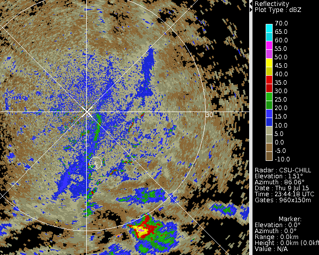
Reflectivity loop
The following reflectivity loop covers the period from 2344 UTC on 9 July to 0052 UTC on 10 July 2015. The time interval between between the images is nominally 1.5 minutes. The motions of the clear air echo patches demonstrate the convergence that was maximized along the fine line echo that was initially located just southeast of the radar. The precipitation shaft from an isolated developing thunderstorm appeared essentially at the Easton site (circled letter E) near 00 UTC. This cell became a part of the large thunderstorm complex that existed in the southeast azimuth quadrant at the end of the loop.
|
|
||
|
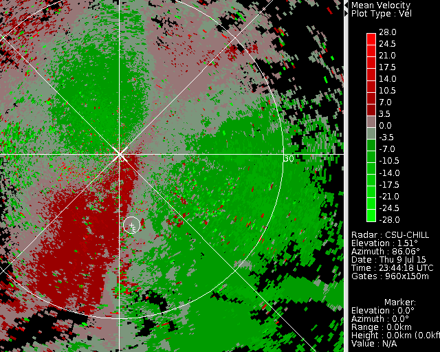
Radial velocity loop
The radial velocity field showed a well-defined convergent pattern in the pre-storm boundary layer. By ~0022 UTC the reflectivity core of the storm that had initially developed over Easton had moved ~4 km to the east of the instrumentation site. The downdraft associated with this echo core began to produce a microburst signature at this time (0022:27 UTC / image frame # 26). With time this microburst pattern expanded and was overtaken by the larger scale outflow pattern associated with the thunderstorm complex near the southern edge of the image frame.
|
|
||
|
Dual polarization radar indications of hail at 9 GHz (X-band)
The CSU-CHILL radar's dual frequency feed horn allows the 9.5 m diameter main reflector to be shared by the 3 GHz and 9 GHz (S- and X-bands respectively) radar systems. This large reflector narrows the 3 dB beam width of the X-band system to 0.33 degrees. The following series of three PPI images show examples of this high resolution X-band data at ~0017 UTC. The reflectivity field contained greater than 50 dBZ intensities in the thunderstorm that was located immediately east of the Easton site:

The correlation coefficient between the co-polar H and V signal returns () decreased to values well below 0.9 in the high reflectivity core. Within heavy thunderstorm precipitation, such correlation reductions are indicative of a broad distribution of hydrometeor shapes, sizes, orientations, and physical composition (i.e., ice vs. liquid water). The diverse hydrometeor populations present in rain - hail mixtures frequently produce local reductions in .


Differential reflectivity () values were distinctly positive (peak values of about +5 dB) in the high reflectivity area near Easton. One source of these large positive Zdr values are small melting hailstones whose spatial orientation is stabilized by a torus of melt water that accumulates around the ice particle's equator.


In combination, the X-band dual polarization measurements suggest that the thunderstorm in the immediate vicinity of the Easton site was generating small, melting hailstones around 0017 UTC. The next section presents selected hydrometeor size, shape, and concentration data collected at the Easton site.
Surface hydrometeor observations at the Easton instrumentation site
The Easton Valley View Airport site has a 2/3rd scaled DFIR double-fence housing several ground based instruments, including a 2D-video disdrometer (2DVD), a droplet spectrometer (MPS), and PLUVIO gage. The three instruments are shown in panel a of Figure 1 shown below. The event had produced large hydrometeors, two example images from the 2DVD are shown in Fig. mt_1(b) and mt_1(c) representing a large drop and a melting hail particle.

Fig. 1: (a) The instrumented site showing the 2/3rd scaled double fence housing the 2DVD, the droplet spectrometer, Pluvio and other instruments, 13 km from CSU-CHILL; (b), (c) 2DVD-based contours of a large rain drop and a melting hail, respectively.
The contour shown in Fig. MT_1(b) is unmistakably that of a raindrop whilst Fig. mt_1(c) differs markedly from it, and may well represent a hail particle at the initial stage of melting where the melting is supposed to occur around the ‘equator’ of the ice sphere. Recently, such hydrometeors have been modeled by a spherical ice-core surrounded by a water toroid, these shapes being based on previously published aircraft probe measurements (silhouettes). Scattering calculations for such hydrometeors have been compared with those for large rain drops at C-band [Thurai, et. al., 2015] using the efficient and accurate higher order method of moments in the surface integral equation formulation [Djordjević and Notaroš, 2004]. The calculations are now being extended to S and X bands in order to compare with the CHILL data for this event (A few other events have also been recorded which had produced hydrometeors with similar 2DVD images to that shown in Fig. mt_1(c)).
The particle size distribution (PSD) derived from the 2DVD measurements are shown as time series in panel a of Figure 2 (shown below). The colors represent the drop concentration for a given (equi-volume diameter) interval over a 1-minute period. Large drops/hydrometeors are seen at the beginning of the microburst event, indicating drop sorting. The full-time PSD for the 30 minute period between 00:00 and 00:30 UTC, i.e. for the entire duration of the event at the instrument site, is shown in Fig. 2(b). Deq values extend up-to 8 mm and higher. The capability of the 2DVD for measuring large drops/hydrometeors has been amply demonstrated in previous studies [Gatlin, et. al., 2015].


Fig. mt_2: (a) Time series of 1 minute PSDs during the microburst event (00:00 – 00:30 UTC) and a second event (02:00 – 02:30 UTC); (b) PSD comparisons; (c) Dm and M corresponding to Fig. mt_2(a); (d) fall velocity versus drop diameter.
Also shown in Fig. mt_2(b) are the 3-minute PSD during the drop-sorting time and a sample 3-minute PSD during the second event which commenced at 02:00 UTC. The distributions have noticeably different shapes. The second event differed from the first (microburst) event in that did not produce hydrometeors larger than 5 mm Deq and it was rain dominated. Fig. mt_2(c) shows the mass-weighted mean diameter (Dm) and the standard deviation of the mass-spectrum (σM) derived from the 1-minute PSDs. At the beginning of the storm, the (unusually) large values of both Dm and σM indicate very wide PSDs. The ratio of the two, i.e. σM / Dm,, is also an important parameter, which has been shown to be in the region of 0.3 [Williams, et. al., 2014] but during the drop-sorting period, this ratio was significantly whereas for other time periods and for the second event, the ratio was closer to 0.3. Fig. mt_2(d) shows the fall velocities versus Deq for the 30-minute period. Altogether, 6263 particles were recorded during the 30 minute time period, and their fall velocities follow the theoretically expected variation. The black curve shown in Fig. mt_2(d) represents the equation [Atlas, et. al., 1973] which is a fit to the well-established Gunn-Kinzer data, but as seen the measurements lie somewhat above this curve. The orange curve represents the corresponding variation after correcting for the reduced pressure at the 1.4 km Greeley altitude. The fall velocity measurements fit this curve significantly better.
References
- [*Atlas, et. al., 1973] Atlas, D., Z. C. Srivastava, and R. S. Sekhon, 1973, Doppler radar characteristics of precipitation at vertical incidence, Reviews of Geophysics, 11, 1–35.
- [*Gatlin, et. al., 2015] Gatlin, P. N., M. Thurai, V. N. Bringi, W. Petersen, D. Wolff, A. Tokay, L. Carey, and M. Wingo, 2015: Searching for Large Raindrops: A Global Summary of Two-Dimensional Video Disdrometer Observations. J. Appl. Meteor. Climatol., 54, 1069–1089.
- [*Djordjević and Notaroš, 2004] Djordjević, M., and Notaroš, B. M., 2004, Double higher order method of moments for surface integral equation modeling of metallic and dielectric antennas and scatterers, IEEE Transactions on Antennas and Propagation, 52, (8), pp. 2118−2129
- [*Thurai, et. al., 2015] Thurai, M., E. Chobanyan, V.N. Bringi and B.M. Notaroš, 2015, Large raindrops against melting hail: calculation of specific differential attenuation, phase and reflectivity, Electronics Letters, 2015, 51, Issue 15, p. 1140 –1142, DOI: 10.1049/el.2015.1564
- [*Williams, et. al., 2014] Williams, C. R., V. N. Bringi, L. D. Carey, V. Chandrasekar, P. N. Gatlin, Z. S. Haddad, R. Meneghini, S. J. Munchak, S. W. Nesbitt, W. A. Petersen, S. Tanelli, A. Tokay, A. Wilson, and D. B. Wolff, 2014: Describing the Shape of Raindrop Size Distributions Using Uncorrelated Raindrop Mass Spectrum Parameters. J. Appl. Meteor. Climatol., 53, 1282–1296.